Introduction

Description

My research focuses on objects called “Manifolds”, which you can think of as higher-dimensional “surfaces”.

• Definition: A Manifold is a space that locally resembles Euclidean space.

One sentence to summarize my research:

• My research explores the “universe” of all possible geometric shapes on manifolds, classifying how complex spaces can collapse into extreme boundaries and proving how they evolve over time to reveal their fundamental structure.

Contents

• Geometry and Topology
• Metric Equivalence
• Moduli space of metrics
• Study of Moduli space: Sequential Limit
• Study of Moduli space: Flow Method

Geometry and Topology

I will introduce two concepts first: Geometry and Topology.

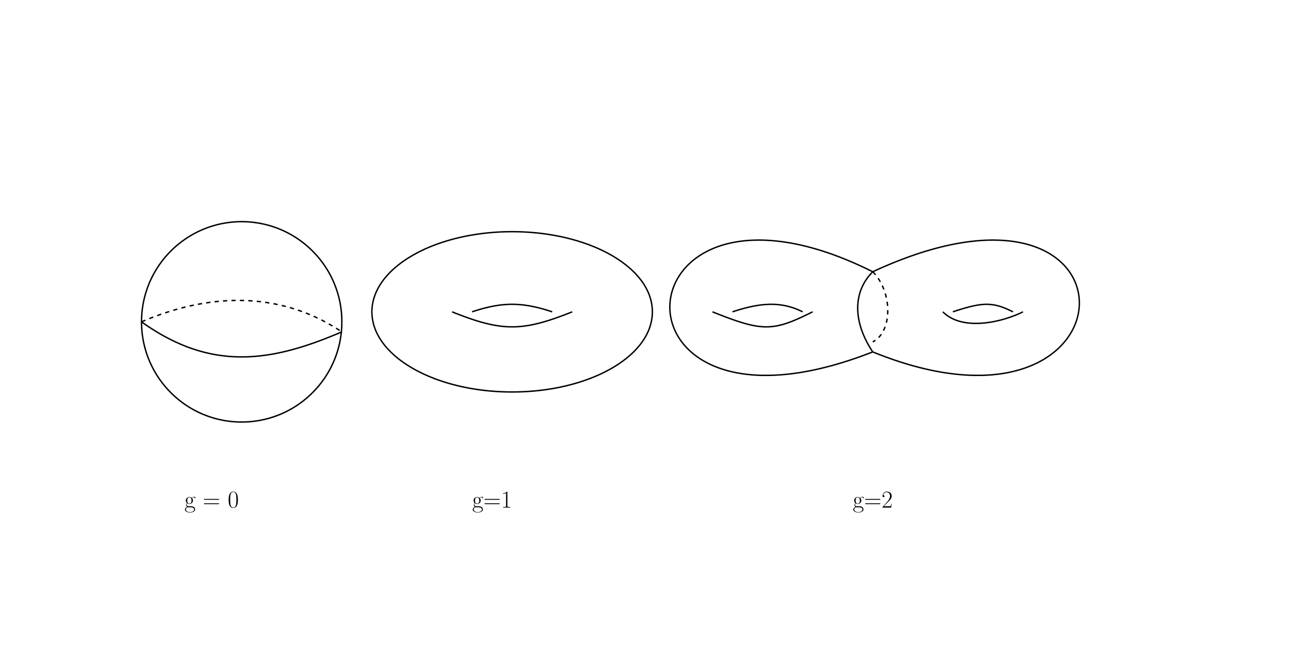
Let’s restrict our discussion to two-dimensional surfaces for now. In dimension one, there is actually no geometry. All closed 1-dimensional curves are just loops; they are equivalent geometrically and topologically. In dimension 2, we call a 2-dimensional manifold a surface. Below are some examples of surfaces.

What is Topology?

Topology is the study of shape in a very relaxed sense. Two objects are topologically the same if you can turn one into the other using only allowed moves. Topology ignores exact sizes and distances. It only cares about connectivity and holes.

Imagine objects made of perfectly stretchy rubber:

• You are allowed to stretch, bend, twist, and squish.
• You are not allowed to:
• tear the object
• glue parts together
• punch new holes

Try the visualization yourself!

You may observe that two closed surfaces are topologically equivalent if they have the same number of “holes”.

This is correct. In dimension 2, the converse is also true:

• If two closed surfaces have the same number of “holes”, they are topologically equivalent.

Thus, the number of holes is a permanent topological fingerprint. Mathematically, this is called Genus, which is the simplest topological invariant.

You can see that topology in this case is “discrete” in nature (Genus allows only non-negative integers).

What is Geometry?

If we view topological properties as “soft”, then Geometry provides the “hard” contrast. In topology, we ignore “wrinkles”, “bumps”, and distortions. But in geometry, these features matter. The most fundamental geometric quantity on a surface is the distance between two points.

How can we define the distance on a surface? Recall that in Euclidean space:

• Among curves connecting two points, the straight line segment is the shortest.

Thus, the distance between two points is defined as the length of the straight line segment connecting them.

On surfaces, we use a similar definition:

• The distance between two points is the minimal length among all curves connecting these two points.

Now we can see an example that distinguishes geometry from topology:

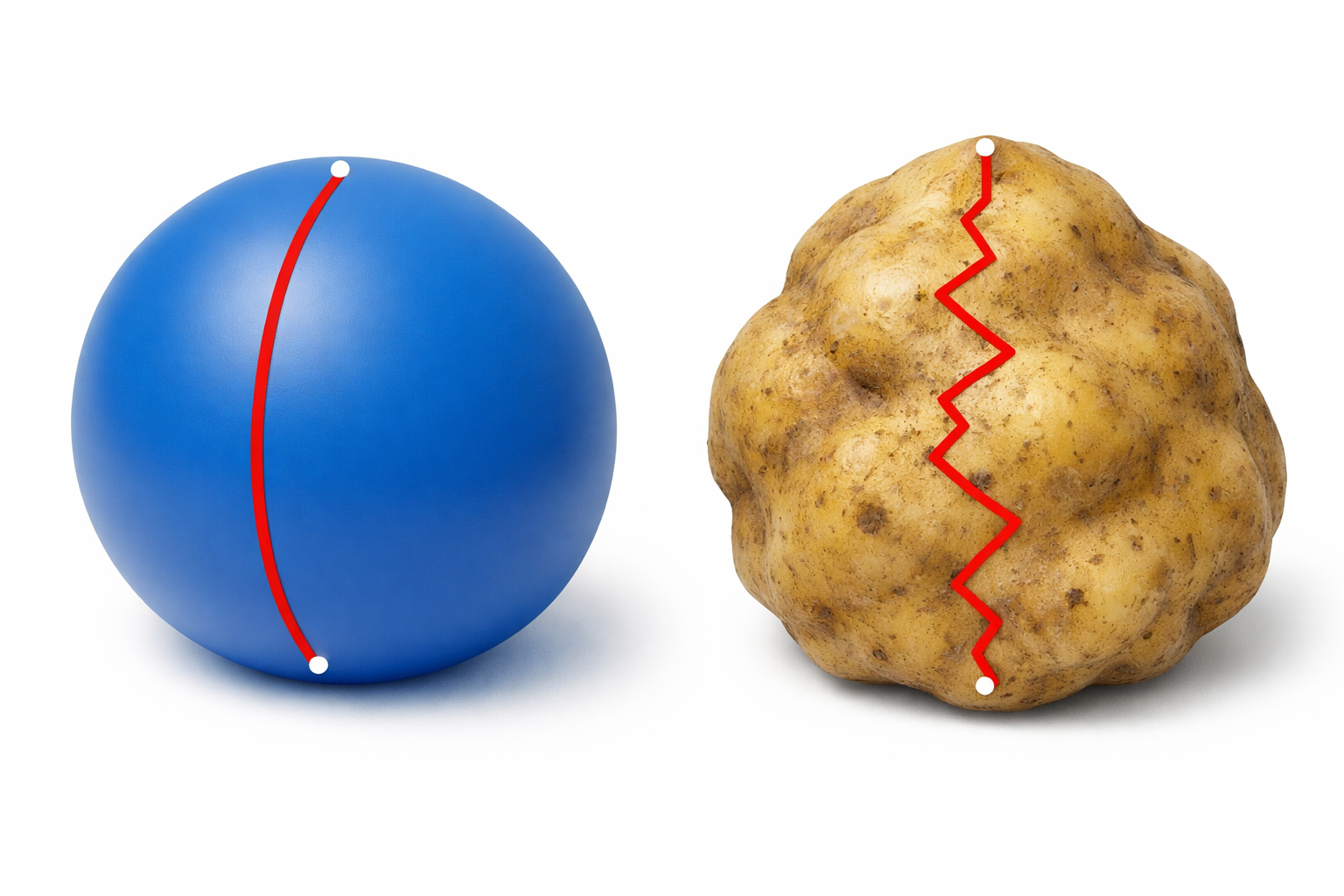
Take the picture above for example. A “sphere” is topologically equivalent to a “potato” (as neither has holes). But the distance between the “north pole” and “south pole” differs. Thus, distance is not a topological property; it is tied to the shape.

We see that different “shapes” determine different distances. We call the “shape” a metric, as it determines distance. In the , you produce many different metrics on the same surface.

Notice that geometry is “continuous” in nature (we can continuously deform a surface’s shape without changing its topology).

Metric Equivalence

As a differential geometer, I am more interested in metrics. We see that a surface can admit many metrics. Here is a big problem:

• How can we distinguish two metrics?

This question is hard. I will answer this question in two steps.

Metric Local Equivalence: Curvature

We can first formulate this locally:

• How can we distinguish two metrics near the same point, say the origin?

Previously, we have seen a metric can determine the distance. But it is a complicated function and not “local” enough. One may think we can let the neighborhood shrink to the origin. However, since a surface is locally “like” Euclidean space $\mathbb{R}^2$, at the origin, it infinitesimally resembles Euclidean space. So distance is not a suitable local invariant.

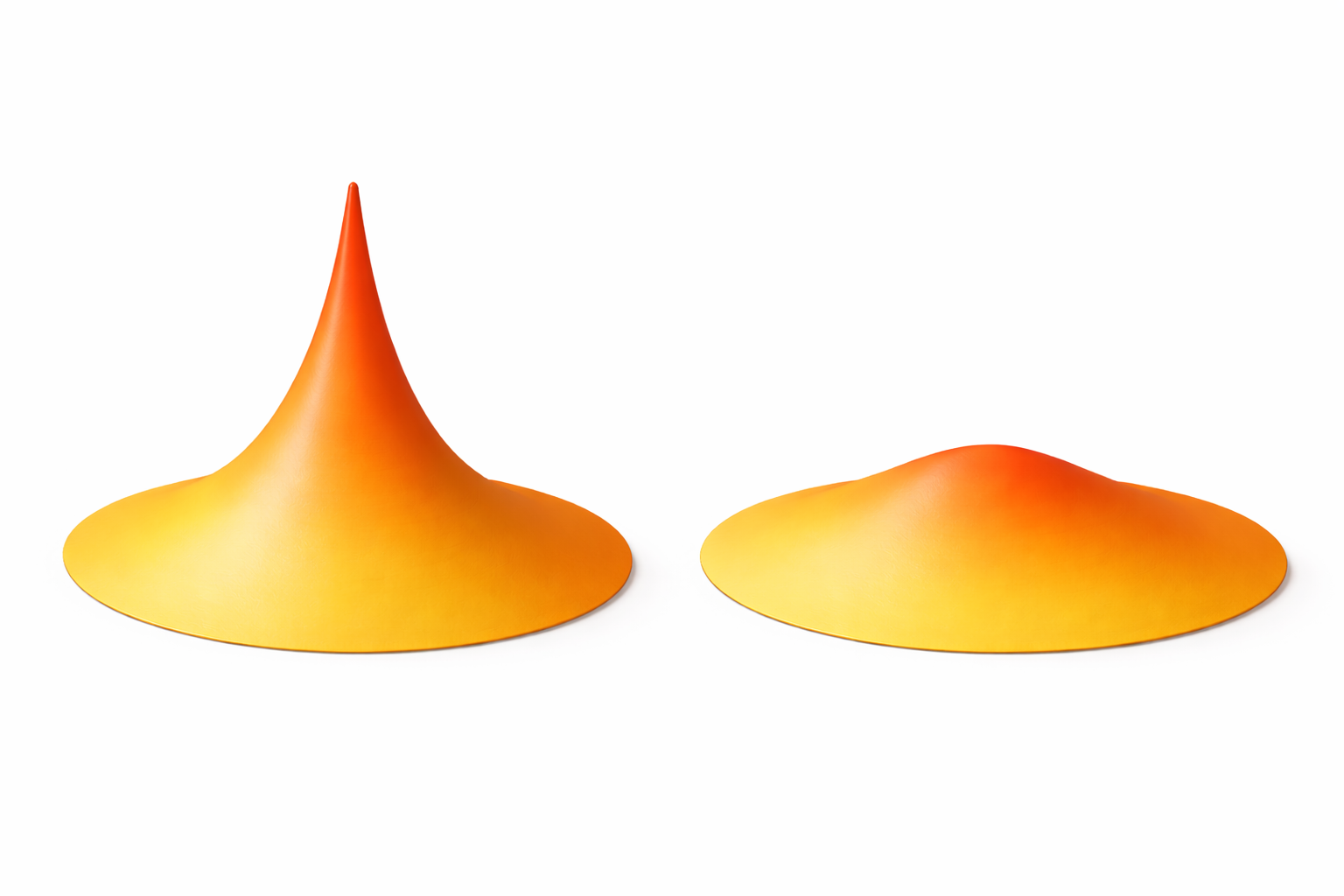
Then, what is the correct invariant? In the picture above, the left surface is “spikier” while the right is “flatter”. In geometry, there is a concept to describe it: curvature.

• Curvature describes how a manifold is “bent” at each point; it is a local invariant.

In the surface case, we can consider “curvature” as a number defined at each point, indicating how “spiky” the surface is around that point.

Global Metric Equivalence

If you agree with this local picture, we can move on to the global question. Consider these two metrics on the sphere:

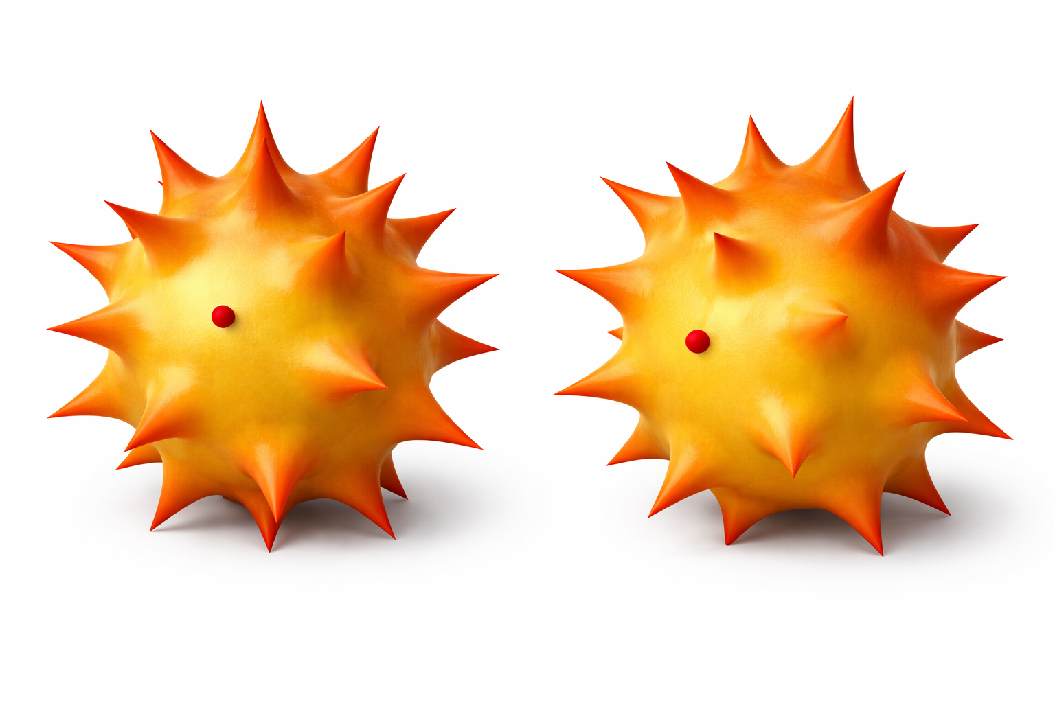
These two “spiky” spheres are effectively the same shape, just rotated. However, if we compare the curvature at a fixed coordinate (e.g., the red dot’s position) on both spheres, the values might differ because the “spike” has moved. Locally, the metrics appear different. But globally, the spheres are isometric—they are the same shape, just rotated.

Motivated by this, we need to carefully define “metric equivalence”.

• Two metrics are equivalent if they are only differed by a “rotation”.

In general, the “rotation” is defined by diffeomorphism.

Now, our metric equivalence definition matches with our intuition. The same spirit holds in physics, where we should always find the quantities that is independent of observors.

Moduli space of metrics

As we have seen, on a surface with fixed the topology, it can admits a lot of metrics, where we count the equivalent metric as one metric. If we put all of these metrics into a space and consider them as whole, it becomes the concept of Moduli space of metrics.

Geometric Application

In the modern view point of geometry, instead of looking at isolated metrics itself, we should regard all of the metrics as a whole and look at its property. Study such moduli space can lead to the answer of the following two core questions of differential geometry:

• Manifold with which topology property can admit certain metric;

• Manifold with which metric must have certain topology property.

For example, in dimension 2, the famous uniformization theorem can be stated.

Theorem

• A closed surface admits a positive constant curvature metric if and on if the genus is 0 (sphere);
• A closed surface admits a zero curvature metric if and on if the genus is 1 (torus);
• A closed surface admits a negative constant curvature metric if and on if the genus is $\geq 2$.

You can image that we need to go and scan the whole moduli space to find such metric. And different underlining topology resulting different moduli space, give us existence and non-existence results.

Distance on Moduli space: Gromov-Hausdorff distance

Here comes the fun part. On a surface, like we have seen, no matter how weird the metric is, we can still measure the distance between two points. One suprising fact is that for two metrics, we can also measure the “distance”. That is to say that we can equip the moduli space with a metric structure. This metric is called Gromov-Hausdorff distance.

The precise definition of Gromov-Hausdorff distance is involved. However, conceptually it is simple. In one sentence:

• Two spaces are close in Gromov–Hausdorff distance if you can match their points so that all distances are almost preserved.

It is still kind of abstract. Let’s see some examples.

The first example: If you still remember the case that two indentical spiky spheres with different rotation angle. Then what is the Gromov-Hausdorff distance? In fact, we can rotate one spiky sphere so that the metric after rotation is a equivalent metric to the other. Thus, their Gromov-Hausdorff distance should be 0. This is intuitively true: since they represent the “same point” in the moduli space, their distance should be 0.

To get a Gromov-Hausdorff distance close example, take a look at this picture: 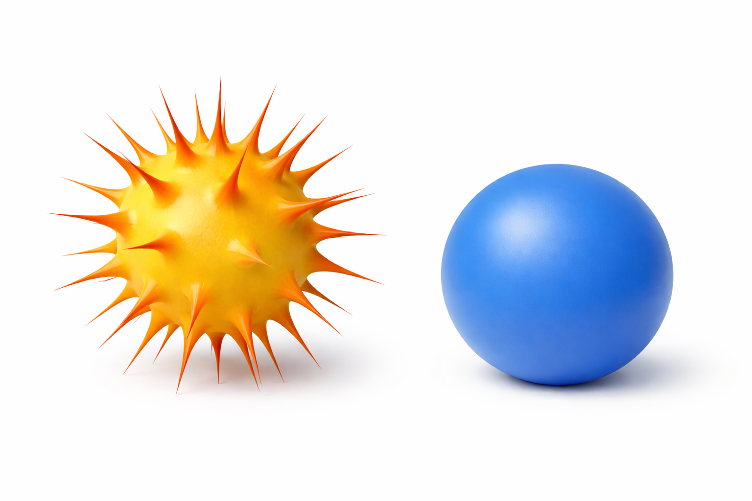The spikes on the left ball is very thin. If we put both spaces into a common “room”, the spherical part are almost identical, which the spikes are almost negligible. Gromov-Hausdorff distance captures global shape while ignoring small geometric noise.

Try this interactive example:

In this example, we can continuosly deform the metric on sphere and torus in the Gromov-Hausdorff sense. Does this looks familar to you? In fact, can be seen in this way:

• the Gromov-Hausdorff distance between the moving metric and the model metric (spherical or standard torus) is becoming smaller and smaller.

A slight difference is that in Gromov-Hausdorff sense, the metric can be closed to a different dimensional space, which means the topology is changed. As the picture shows, torus can “collapse” to a circle, which is a lower dimensional space.

Intuitively speaking,

• What you look like close are close in Gromov-Hausdorff distance.

Study of Moduli space: Sequential Limit

Finally, I can introduce my research part.

Like I said, my research focus on the moduli space of metrics. I mainly work on higher dimension spaces, so let’s restore the terminology “manifold”.

One interesting question is:

• What is the boundary of the moduli space?

We have introduced the Gromov-Hausdorff distance. To say “boundary”, which is like a finite distance thing, so we may need to impose some “conditions” on the metrics and consider a “subset” of metrics to avoid distance tends to infinity. I worked on a subset of the moduli space whose metrics satisfies a very natural “condition” in high dimension.

A way to understand the boundary is to find a sequence of metrics to approach to the boundary. Like in the real number, we can take a limit. Under Gromov-Hausdorff distance, we can also take a limit. But the problem is that, the limit may not be “manifold” anymore. Metric degenerations can happen, and topology will change. The “collapsing” is one type of degenerations. There are a lot of degenerations which are unknown. So one of my work can be stated in this way. See details in my research.

• Theorem Consider the moduli space satisfies the natural “condition”,
  • If we assume they are not “collapsing”, in dimension 3 and 4, all of the “boundaries” are classified. In any dimension, the classification of the “boundaries” becomes an “algebraic” (group theory) problem.
  • If we allow “collapsing”, new examples are discovered.

An illustration of this new examples is like the one in my homepage:

We can see the left manifold is roughly “unchanged”, while the right manfiold is “collapsing” to lower dimension. The “linking neck” region is shrinking to a point.

A fun fact is that the “linking neck” region is actually a Schwarzschild_metric, which is actually a mathematical model for the black hole.

Study of Moduli space: Flow Method

Another way to study the moduli space is to using the so-called “flow method”. The most famous flow among others is Ricci flow.

“Flow method” often seeks the answer to the above two questions:

• Manifold with which topology property can admit certain metric;

• Manifold with which metric must have certain topology property.

Let’s mainly focus on Ricci flow and ponder the question.

• Why Ricci flow is a suitable “weapon” to answer the above two question?

For every point on a manifold, there is a curvature, which at the begining, could be different for different points. Image the manifold is like a closed chamber and the curvature is like “heat” distribution. If there is no other heat source, the heat distribution will be more and more “homogeneous”, and eventually, the heat will be evenly distributed in the chamber. Ricci flow is an analog of the heat flow. Idealy, it will make everywhere on the manifold the constant curvature.

You may recall this picture:

On 2 dimension sphere, you can see the “bumps” are like the curvature distribution on sphere, and Ricci flow will make the high and low curvatrue region more “spherical”. In the end, it will get the desired metric with constant curvature everywhere, the round metric. With some proof, we can say:

• A 2 dimension sphere (topological condition) admit a positive constant curvature metric.

However, this intuition fails in 3 and higher dimension. The biggest issue is that “singularity” will occure, and prevent the flow to extend further. What I mean “singularity” is the place where curvature tends to infinity. This does not happen in the heat flow, but inevitable in Ricci flow. That is why it took a generation to fully solve the Poincaré conjecture, the main difficulty is how to deal with singularites. The whole proof basically can be summerized into two steps.

• A 3 dimensional “simply connected” manifold admit a metric that Ricci flow with surgery that will terminate in finite time for all componenents.
• A 3 manifold admit a metric that Ricci flow with surgery that will terminate in finite time for all componenents must be a 3 dimensional sphere.

Here is an illustration of what is happening if you start a Ricci flow with a “simply connected” 3 manifold.

To wrap it up, Ricci flow solves a pure topological conjecture, which is very impressive. I will write “A higher level introduction to Poincaré conjecture” in the future.

Now, I want to summerize what I have done. We consider a flow which is very natural and closed related to Ricci flow. We call this $\alpha$-Ricci flow. Me and my coauthors show the following results (we are still working on some part of the proof).

• Theorem Consider the $\alpha$-Ricci flow.
  • The $\alpha$-Ricci flow on 2-torus will either “collapse” to a circle or to a point in the Gromov-Hausdorff distance, depending on a rationality condition initially;
  • The $\alpha$-Ricci flow with surgery on some 3 manifold will exist forever and converge to the desired metric in the Gromov-Hausdorff distance.

If you are interested in the details, please take a look at my research.